Lesson 14: Year 11 Catch-Up
Data, Structures & Tools — the 16 things that weren't on your radar yet
1 — Number Systems & Data Representation ~20 min
Why computers think in binary
Every transistor in a processor is either on (1) or off (0). Everything on a screen — text, images, video — is ultimately a long sequence of 1s and 0s. Understanding how numbers are represented lets you understand how data is stored, transmitted, and sometimes corrupted.
The three bases NESA
| Base | Name | Digits used | Where you see it |
|---|---|---|---|
| Base 2 | Binary | 0, 1 | CPU registers, file storage, network packets |
| Base 10 | Decimal | 0–9 | Everywhere in daily life |
| Base 16 | Hexadecimal | 0–9, A–F | Colour codes, memory addresses, hash outputs |
Binary ↔ Decimal NESA
Each binary digit (bit) has a positional value that doubles as you move left: 1, 2, 4, 8, 16, 32, 64, 128…
Hexadecimal NESA
Hex is a shorthand for binary. Every 4 bits maps to exactly one hex digit — so an 8-bit byte becomes two hex characters. This is why memory addresses and colour codes are written in hex.
| Decimal | Binary | Hex |
|---|---|---|
| 0 | 0000 | 0 |
| 9 | 1001 | 9 |
| 10 | 1010 | A |
| 15 | 1111 | F |
| 255 | 1111 1111 | FF |
💡 Hex in practice
CSS colour #DD6B20 is hex. Break it down: DD = red (221), 6B = green (107), 20 = blue (32). Every colour on screen is stored as 3 bytes of binary data.
Two's Complement — representing negative numbers NESA
Computers can only store 0s and 1s. So how do they store −37? The answer is two's complement.
The process: three steps
- Write the positive version in binary. +37 in 8-bit binary =
00100101 - Flip every bit (invert).
00100101→11011010 - Add 1.
11011010+00000001=11011011
So −37 is stored as 11011011. You can verify: if the leading bit is 1, the number is negative.
Why two's complement?
- Only one representation of zero (avoids +0 and −0 ambiguity)
- Normal binary addition works for both positive and negative — no special hardware needed
- For 8 bits: range is −128 to +127
▶ Challenge: find two's complement of −12
+12 = 00001100 → flip → 11110011 → add 1 → 11110100
⬡ Beyond NESA: why adding two's complement numbers works
+37 = 00100101, −37 = 11011011. Add them: 00100101 + 11011011 = 100000000 — that's a 1 followed by 8 zeros. Drop the overflow bit and you get 00000000 = zero. The math just works, which is why every CPU uses two's complement.
Real and floating point data types NESA
You already know int (whole numbers) and str. Here are the two decimal types:
| Type | Meaning | Example values | Python keyword |
|---|---|---|---|
| Real | Any number with a decimal point — rational or irrational | 3.14, −0.5, 2.718… | float |
| Single precision float | Real stored in exactly 32 bits using IEEE 754 format | stored as sign + exponent + mantissa | C's float, Python's float is actually 64-bit |
⚠️ The float precision trap
Not every decimal can be represented exactly in binary.
print(0.1 + 0.2)          # You'd expect 0.3
# Actual output: 0.30000000000000004

# Why? 0.1 and 0.2 can't be stored exactly in binary.
# They're stored as the closest representable value.

# Fix: use round() when comparing decimals
print(round(0.1 + 0.2, 1) == 0.3)   # True
⬡ Beyond NESA: IEEE 754 — what's inside a 32-bit float
A single-precision float uses 32 bits split into three parts:
- 1 bit — sign (0 = positive, 1 = negative)
- 8 bits — exponent (biased by 127)
- 23 bits — mantissa (the significant digits)
Value = (−1)^sign × 1.mantissa × 2^(exponent−127). This is why precision problems exist — you're forcing an infinite decimal into 23 bits.
2 — Data Structures: Records, Trees & Files ~25 min
Records NESA
A record represents a single entity with named fields — like one row in a spreadsheet. Unlike an array (which uses integer indices), a record lets you access data by a meaningful name.
Array approach (less readable)
student = ["Blake", 17, "Year 12"]
# Access by position — fragile
name = student[0]
Record approach (named fields)
from dataclasses import dataclass

@dataclass
class Student:
    name: str
    age: int
    year: str

student = Student("Blake", 17, "Year 12")
print(student.name)  # "Blake"
In Python you can also use a plain dict as an informal record: student = {"name": "Blake", "age": 17}. The dataclass is the more formal, type-safe version.
💡 Record vs Array — the key distinction
Arrays hold multiple values of the same type accessed by index (position). Records hold multiple related fields with different types accessed by name. A record describes one thing; an array describes many of the same thing.
Trees NESA
A tree is a hierarchical data structure — data is organised in a parent-child relationship. Unlike a linked list (one chain), a tree branches.
Vocabulary
| Term | Meaning |
|---|---|
| Root | The top node — no parent |
| Parent / Child | Every node (except root) has one parent; a node can have multiple children |
| Leaf | A node with no children — at the bottom of the tree |
| Subtree | Any node plus all its descendants |
| Height | Number of edges from root to deepest leaf |
Binary Search Tree (BST) — a common form NESA
In a BST, every node satisfies one rule: left child < parent < right child. This means searching is fast — at each node you can immediately discard half the tree.
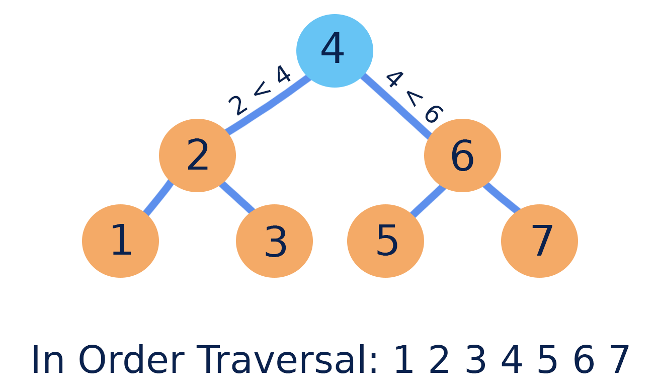
BST containing: 4, 2, 6, 1, 3, 5, 7 — in-order traversal yields sorted output: 1 2 3 4 5 6 7
Implementing a BST node in Python NESA
class Node:
    def __init__(self, value):
        self.value = value
        self.left = None    # smaller values go left
        self.right = None   # larger values go right

class BinarySearchTree:
    def __init__(self):
        self.root = None

    def insert(self, value):
        if self.root is None:
            self.root = Node(value)
        else:
            self._insert_recursive(self.root, value)

    def _insert_recursive(self, node, value):
        if value < node.value:
            if node.left is None:
                node.left = Node(value)
            else:
                self._insert_recursive(node.left, value)
        else:
            if node.right is None:
                node.right = Node(value)
            else:
                self._insert_recursive(node.right, value)

bst = BinarySearchTree()
for v in [4, 2, 6, 1, 3, 5, 7]:
    bst.insert(v)
💡 Trees are everywhere
A file system is a tree. The browser's DOM is a tree — <html> is the root, <body> is a child, each element is a node.
⬡ Beyond NESA: BST vs balanced trees (AVL, Red-Black)
A BST degrades to a linked list if you insert already-sorted data (1, 2, 3, 4… all go right). Balanced trees (AVL, Red-Black) automatically reorganise to keep height minimal — guaranteeing O(log n) search always, not just on average.
Sequential Files NESA
A sequential file stores records one after another in a fixed order. To find a record, you start at the beginning and read forward — you can't jump to record 500 without passing records 1–499 first.
In Python: CSV as the classic example
import csv

# Sequential: we must read every row from top to bottom
with open("students.csv", "r") as f:
    reader = csv.reader(f)
    for row in reader:          # row 1, then 2, then 3...
        print(row[0], row[1])   # name, grade

# To find one student, you still read the whole file
# (unless you know the line number — which is unusual)| Sequential File | Random Access File | |
|---|---|---|
| Access pattern | Read from start in order | Jump to any record by index |
| Example | CSV, log files, audio streams | Binary files with fixed-size records |
| Best for | Processing all records, append-only logs | Frequent lookup by position |
Stack & Hash Table implementations NESA
Stack NESA
A stack is LIFO — Last In, First Out. Items are pushed onto the top and popped from the top. The classic analogy is a stack of plates.
class Stack:
    def __init__(self):
        self._items = []

    def push(self, item):
        self._items.append(item)    # add to top

    def pop(self):
        if self.is_empty():
            raise IndexError("Stack is empty")
        return self._items.pop()    # remove from top

    def peek(self):
        return self._items[-1]      # view top without removing

    def is_empty(self):
        return len(self._items) == 0
Hash Table NESA
A hash table stores key-value pairs and achieves near-constant-time lookup. It works by running the key through a hash function that converts it to an array index.
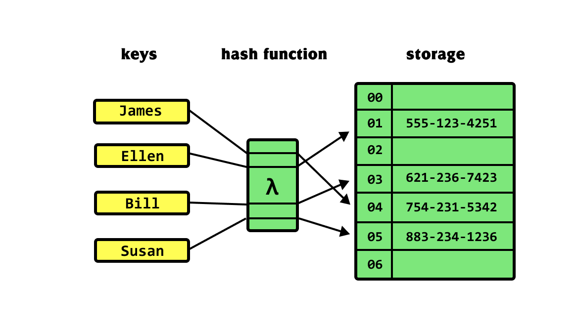
Keys (names) → hash function → array index → stored value (phone number). Each key maps to a specific slot.
# Python's dict IS a hash table — O(1) average lookup
phonebook = {
    "Blake": "0411 000 111",
    "Luis":  "0422 000 222",
    "Jogo":  "0433 000 333",
}

# Lookup: Python hashes "Blake" to find the right slot instantly
print(phonebook["Blake"])   # O(1) — same speed whether 10 or 10,000 entries

# Manual hash table (to understand what dict does under the hood)
class SimpleHashTable:
    def __init__(self, size=10):
        self.table = [None] * size

    def _hash(self, key):
        return sum(ord(c) for c in key) % len(self.table)

    def set(self, key, value):
        index = self._hash(key)
        self.table[index] = (key, value)

    def get(self, key):
        index = self._hash(key)
        entry = self.table[index]
        if entry and entry[0] == key:
            return entry[1]
        return None
⬡ Beyond NESA: hash collisions
Two different keys can produce the same hash index — called a collision. Real hash tables handle this with chaining (each slot holds a linked list of entries) or open addressing (probe the next empty slot). Python's dict uses a sophisticated open-addressing scheme.
3 — Algorithm Modelling Tools ~15 min
Structure charts & refinement diagrams NESA
You've used flowcharts to show how code runs step-by-step. Structure charts show something different: what modules exist and which ones call which.
| Flowchart | Structure Chart | |
|---|---|---|
| Shows | Control flow (sequence, selection, iteration) | Module hierarchy (which calls which) |
| Shapes | Diamonds (decisions), rectangles (steps), arrows | Rectangles (modules), lines with arrows showing calls |
| Best for | Explaining a single algorithm's logic | Designing the structure of a whole program |
Structure chart example

Structure chart — login system. Arrows show which module calls which, not control flow.
Refinement diagrams NESA
A refinement diagram is how you design top-down — start with a vague high-level step, then break it down. Each box gets "refined" into smaller boxes until every box is simple enough to code directly.

Stepwise refinement — each level decomposes the level above until every box is one simple function.
💡 The key insight
Structure charts are drawn before you write code — they're a design tool. Once you have a structure chart, each box becomes a function or method. The connections tell you what parameters to pass and what to return.
Subroutine connections — data flow in algorithms NESA
When one algorithm calls another, there are two things flowing between them:
- Parameters — data passed into the called subroutine (going down in the structure chart)
- Return values — data passed back to the caller (going up)
def calculate_total(items: list) -> float:
    """Called by: checkout_process. Receives: list of prices. Returns: total."""
    subtotal = sum(items)
    return apply_discount(subtotal)     # calls another subroutine

def apply_discount(amount: float) -> float:
    """Called by: calculate_total. Receives: subtotal. Returns: discounted price."""
    if amount > 100:
        return amount * 0.9             # 10% discount
    return amount

def checkout_process(cart: list) -> None:
    """Top-level. Calls: calculate_total."""
    total = calculate_total(cart)       # data flows down (cart → items), up (total ← return)
    print(f"Total: ${total:.2f}")
🗂️ Challenge: draw the structure chart
For the code above, draw a structure chart showing the three modules. Indicate what data passes down (as parameters) and what comes back up (as return values) on each connecting line.
▶ Show answer
checkout_process → calls calculate_total (passes: cart, receives: total) → calls apply_discount (passes: subtotal, receives: discounted amount)
4 — Standard Modules, Testing & IDE Debugging ~20 min
Standard modules NESA
A standard module is pre-written, pre-tested code that ships with Python — no installation needed, just import. They exist so you never have to reinvent the wheel for common tasks.
| Module | What it does | Example use |
|---|---|---|
math | Mathematical functions | math.sqrt(144), math.pi, math.floor(3.7) |
random | Random number generation | random.randint(1, 6) (dice roll), random.shuffle(deck) |
datetime | Dates and times | datetime.date.today(), datetime.timedelta(days=7) |
os | File system and OS interaction | os.path.exists("file.txt"), os.getcwd() |
csv | Read/write CSV files | csv.reader(f), csv.writer(f) |
json | Encode/decode JSON | json.dumps(data), json.loads(text) |
import math
import random
import datetime

# math
radius = 5
area = math.pi * radius ** 2
print(f"Circle area: {area:.2f}")      # 78.54

# random
dice = random.randint(1, 6)
print(f"You rolled: {dice}")

# datetime
today = datetime.date.today()
due_date = today + datetime.timedelta(days=14)
print(f"Assignment due: {due_date}")
🌋 Volcanic Pantheon connection
Your my_api.py file in BlakeLovesJogo is essentially a hand-written standard module — greet(), shout(), add(), multiply(). The only difference from Python's math module is that math was written by the Python core team and ships everywhere. The concept is identical: import it, call its functions, done.
Path coverage testing NESA
You already know boundary value testing (test at edges: 0, max, one below max). Path coverage is a different idea: every possible branch through the code must be executed by at least one test case.
def classify_score(score: int) -> str:
    if score >= 90:          # branch 1: True / False
        return "HD"
    elif score >= 75:        # branch 2: True / False
        return "Distinction"
    elif score >= 50:        # branch 3: True / False
        return "Pass"
    else:
        return "Fail"
❌ Insufficient — boundary only
Test: score = 90 (edge of HD)
Test: score = 0 (minimum)
Misses the Distinction and Pass branches entirely.
✅ Path coverage — all branches hit
Test 1: score = 95 → "HD" (branch 1 True)
Test 2: score = 80 → "Distinction" (branch 2 True)
Test 3: score = 60 → "Pass" (branch 3 True)
Test 4: score = 40 → "Fail" (else branch)
💡 Boundary vs Path coverage — when to use each
Boundary testing checks that edge values don't crash or give wrong results. Path coverage ensures every branch of your logic has been exercised at least once. A good test suite does both.
▶ Challenge: how many test cases does path coverage require for this function?
def check_login(username, password, is_admin):
    if username == "":
        return "error: no username"
    if password == "":
        return "error: no password"
    if is_admin:
        return "admin dashboard"
    return "user dashboard"
Answer: 4 test cases — empty username, empty password, is_admin=True (with valid credentials), is_admin=False (with valid credentials). Each covers a distinct path through the function.
Debugging interfaces between functions NESA
Most bugs don't live inside a function — they live at the boundary between functions. The caller passes the wrong type, or the wrong shape of data, or the callee returns something the caller doesn't expect.
def get_student_average(scores: list) -> float:
    return sum(scores) / len(scores)

def grade_student(student_name: str, scores) -> str:
    avg = get_student_average(scores)
    if avg >= 50:
        return f"{student_name}: Pass"
    return f"{student_name}: Fail"

# Bug: scores was accidentally passed as a string, not a list
result = grade_student("Blake", "85 90 78")
# get_student_average receives "85 90 78" (a string, not a list)
# sum("85 90 78") → TypeError  ← the error is at the interface

# How to debug interfaces: check what you're sending IN and getting back OUT
print(type(scores))          # see what's actually arriving
print(repr(scores))          # see the exact value
# Or use a debugger breakpoint right at the function call
When a function produces unexpected results, check what is being passed in first — not just what happens inside it.
IDE debugger NESA
Most IDEs include a built-in debugger that is faster and cleaner than inserting print() statements — and leaves no debug output in finished code.
The three tools you need to know
| Tool | What it does | Better than print because… |
|---|---|---|
| Breakpoint | Pauses execution at a line you choose — click the gutter (line numbers area) in VSCode | No code to add/remove; pause exactly where you want |
| Step Over (F10) | Execute one line, stay at the same level — don't descend into function calls | See line-by-line what happens without print everywhere |
| Step Into (F11) | Execute one line and descend into the function call — follow the code into the subroutine | Inspect what happens inside a function call without modifying it |
Watches
In the Variables and Watch panel, type any expression and see its value update in real time as you step through code — every variable simultaneously, without writing a single extra line.
💡 How to set a breakpoint in VSCode
1. Open your Python file → hover over the grey area left of a line number → a red dot appears → click it to set the breakpoint.
2. Press F5 (Run and Debug) instead of the normal Run button.
3. Execution pauses at your breakpoint — all variable values are visible in the left panel. Use F10 to step line by line.
✅ Year 11 foundations: complete
This lesson covers the remaining Year 11 Programming Fundamentals topics:
- Number systems: Binary, decimal, hex — conversions in both directions
- Two's complement: How computers store negative numbers and why
- Real vs float: What single-precision means and why 0.1 + 0.2 ≠ 0.3
- Records: Named fields for a single entity (contrast with arrays)
- Trees & BSTs: Hierarchy, root/leaf, left < parent < right, O(log n) search
- Sequential files: Top-to-bottom access, CSV as the canonical example
- Stacks & hash tables: LIFO push/pop, dict as a hash table under the hood
- Structure charts: Module hierarchy (not flow), useful before you write any code
- Subroutine connections: What data passes in (parameters) and out (return values)
- Standard modules: math, random, datetime — import and use
- Path coverage: Every branch must be hit by at least one test case
- Interface debugging: Check what you pass in, not just what happens inside
- IDE debugger: Breakpoints, step over, step into, watches — no more print spam
Next up → Lesson 15: Client-Server Architecture & APIs